Dan Sullivan

Design and Control of an Inverted Pendulum

1. Summary

The control of an Inverted pendulum is a well studied problem in controls engineering. While the system dynamics are non-linear, the dynamics can be linearized so that simple, linear control algorithms such as PID and full state feedback can be used to stabilize the non-linear system. I began this project to solidify my knowledge of classical control theory as well as develop a system where I could begin to investigate more complicated, non-linear control algorithms.

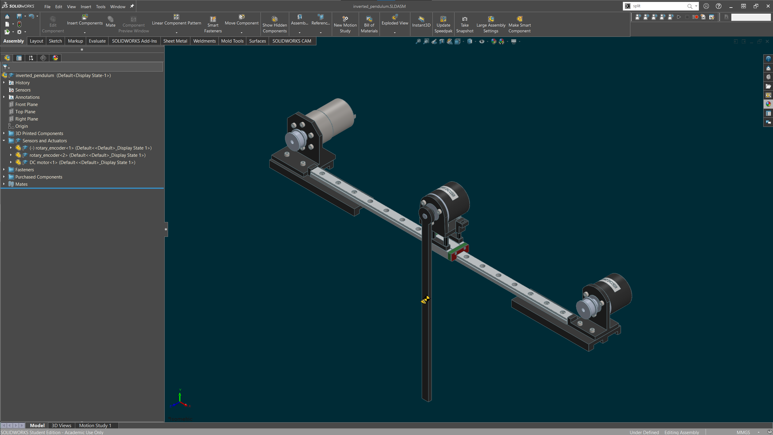
After 3 months of work, I was able to have a working plant and control system:

2. System Design

The mechanical design of the pendulum was relatively straightforward. Many inverted pendulum systems are viewable on the internet and I drew on these for inspiration.

For this system, I chose to place the pendulum on a cart secured to a track. Other inverted pendulum systems mount the pendulum on a rotary table, or a moving cart itself. The fixed cart-pendulum design appeared the most straightforward.

For sensors and actuators, I chose to go with incremental rotary encoders and a brushed DC motor. Incremental rotary encoders allowed for the high-resolution angle sensing that I desired and were also relatively inexpensive. While I may have selected a stepper motor or brushless DC motor, I chose a brushed DC motor as it did not require complex driver boards or circuitry.

The mechanical design of the system in SolidWorks is shown below:

SolidWorks Design

3. System Modeling

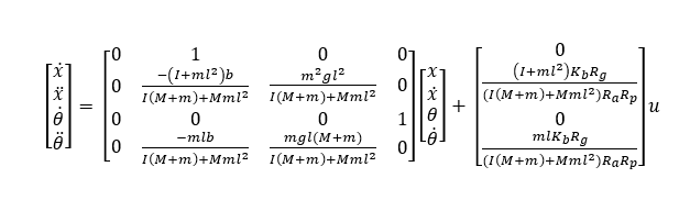
Modeling the system dynamics of the cart-pendulum system is more challenging than the introductory control systems taught during undergraduate control classes. The non-linearity introduced by gravity and the angle of the pendulum leads to an interesting system of differential equations. Additionally, when modeling the real cart-pendulum system, it is possible to have an extremely detailed model with many additional state variables and non-linearities, increasing the complexity of the system dramatically. For example, the inertial elements of the gear-train within the motor, inertia of the timing belt, compliance of the timing belt, and gear backlash, are all complex dynamics which are part of the real pendulum system, but not accounted for within simple models.

I may create a more complex system model in the future development of this pendulum system, but for the purposes of initially controlling this system, I chose to develop the state space with 4 state variables: the position of the cart, velocity of the cart, the angular position of the pendulum, and the angular velocity of the pendulum.

The state space derived for this system is shown below:

The variables in the state space above correspond to the following variables:

Variable	Description	Variable	Description
θ	Pendulum angle	g	Gravitational acceleration
x	Cart position	Kb	Motor torque constant
M	Cart mass	Rg	Gear ratio
m	Pendulum mass	Ra	Motor armature resistance
b	Rail friction	Rp	Timing pulley radius
I	Pendulum moment of inertia	u	Motor input voltage

The majority of the system parameters were easily measurable. The motor armature resistance, and rail friction, were harder to calculate. I estimated these parameters by using basic system identification techniques; simulated system dynamics were compared to measured system dynamics and the parameters were updated and tuned until the simulated and real dynamics matched.

4. Control Software Development

With the physical system built, and the system model fully developed, I began writing the control software in C with Atmel Studio for an Arduino target. A state-machine structure was chosen for simplicity. The current states of the pendulum system are 1) rest and 2) active control. A hardware button transitions in-between the two. The active control state will attempt to control the pendulum to the point held during the rest state. Basically, the rest state is used to position the pendulum upright, and in the center of the track, and then the active control state uses the calculated rotary encoder positions for setpoints. All code written is available at the GitHub repository here. The code is divided between 3 main files. "main.c" contains the state machine structure, functions for USART communication with an external PC, and a function for software-debouncing of input buttons. "hardware.c" includes driver functions operating the external DC motor control board, as well as performing register setup for the arduino board. "hardware.c" could be refactored for use on different target microcontrollers. "control_functions.c" contains the P, PI, PID, and LQR control functions. Interesting sections of code are outlined below.

LQR Feedback Calculation


   double* LQR(double* x_error, double* xdot_error, double* theta_error, double* thetadot_error){
       
       //Calculate the LQR with gain array K and passed errors
       LQR_value = -(K[0]*(*x_error) + K[1]*(*xdot_error) + K[2]*(*theta_error) + K[3]*(*thetadot_error));
       return &LQR_value;
   
   }

The LQR feedback method, located in "control_functions.c" is the implementation of the full-state feedback with control gains K calculated from MATLAB. The MATLAB Code used to calculate the control gains is shown below.

LQR Feedback MATLAB Calculation


   %% LQR calculation
   
   %System parameters
   l_com = 0.11302;    %[m] - distance to the center of mass of the pendulum
   m_cart = 0.169;     %[kg] - mass of the cart
   m_pendulum = 0.016; %[kg] - mass of the pendulum
   R_armature = 6.5;       %[Ohm] - armature resistance of the motor
   b_rail = 0.0000005; % rail friction coefficient (estimated with system identification)
   I = 0.000089809; 
   g = 9.81;
   R_pulley = 0.0095504;   %[m] - pulley radius
   gear_ratio = 5000 / 550;
   Kb = 0.059682;          %motor constant
   
   Denom = I*(m_cart+m_pendulum) + m_cart*m_pendulum*l_com^2; %common denominator in calc
   
   A = [0 1 0 0;
        0 -(I + m_pendulum*(l_com^2))*b_rail/Denom (m_pendulum^2)*g*(l_com^2)/Denom 0;
        0 0 0 1;
        0 -m_pendulum*l_com*b_rail/Denom m_pendulum*g*l_com*(m_cart+m_pendulum)/Denom 0];
    
    B = [0;
         (I + m_pendulum*(l_com^2))*Kb*gear_ratio/(R_armature*R_pulley*Denom);
         0;
         m_pendulum*l_com*Kb*gear_ratio/(R_armature*R_pulley*Denom)];
   
   Q = [10 0 0 0;
           0 0.02 0 0;
           0 0 40 0;
           0 0 0 0.0001];
       
   R = 0.0001;
   
   k = lqr(A, B, Q, R)
   
   C = [1 0 0 0];
   D = 0;
   
   closed_pendulum_sys = ss(A-B*k, B, C, D)
   pzmap(closed_pendulum_sys)

With the MATLAB library function "lqr", LQR control gains can be calculated quite easily. I chose to use a continuous LQR system, as the loop speed appears fast enough to ignore discrete control effects. The "Q" matrix assigns cost to the error of each of the state variables. As you can see, my "Q" matrix heavily assigns cost to error in the position of the cart, and the angle of the pendulum, but not their derivatives - this allows for strong feedback gains, and low derivative feedback gains. The R matrix (scalar in this problem, as there is only 1 system input) assigns "cost" to the motor input. I chose a low value for the R matrix as I do not care about the system over-actuating, I care more about the system remaining stable (besides, a single DC motor does not cost that much to operate).

Rotary Encoder Interrupt Service Routine


   ISR(PCINT2_vect){
       
       static const int8_t rot_states[] = {0, -1, 1, 0, 1, 0, 0, -1, -1, 0, 0, 1, 0, 1, -1, 0};
       static uint8_t AB[2] = {0x03, 0x03};  //for storing old and new values of pins
       uint8_t t = PIND;                      //read Port B
       t = (t >> 2) & 0b00001111;								//used to keep dig pin 0/1 open for TX/RX in futue
       
       //check for rotary state change
       AB[0] <<= 2;       //save previous state (by bit shifting it left)
       AB[0] |= t & 0x03; //add the new state to the 2 LSB of AB (by making this the 2 LSB)
       rot_pendulum += rot_states[AB[0] & 0x0f]; //increment or decrement the rotation
       
       AB[1] <<= 2;		//save previous state
       AB[1] |= (t >> 2) & 0x03; //shift t to the right two (move 2nd r.e. inputs to the LSB) 
       rot_cart += rot_states[AB[1] & 0x0f]; //increment or decrement
   }

This method is located within "main.c". Both incremental rotary encoders are connected to this ISR, so one rotary encoder change will trigger this method to update both of their positions. This ISR has the variable AB[], used to store the past and present states of the A/B signal lines for both rotary encoders. The past and present values can be stored with 4 bits of information - for a total of 16 different combinations of past/present signal values. The rot_states variable represents the proper increment and decrement step for each of these combinations of A/B values.

State 1 Loop


   while(state == 1){
               
       //continue to debounce the state transition button
       debounce();
               
       //measurement estimates
       angle = (double)rot_pendulum * angle_conversion_factor_rads;
       position = (double)rot_cart * position_conversion_factor;
               
       get_time_information();
               
       moving_average_derivative_calculation();
               
       save_previous_states();
               
       calculate_error();
                       
       //CONTROLLERS
                   
       //P Controller
       //compare_register_set = motor_feedback_control(P(&angle));
               
       //PI Controller
       //compare_register_set = motor_feedback_control(PI(&angle, &dt));
                   
       //LQR Controller
       compare_register_set = motor_feedback_control(LQR(&x_error, &xdot_error, &theta_error, &thetadot_error));
       OCR1A = compare_register_set;
               
       
   }

This code is the active control state of the pendulum. At the beginning of each state within "main.c", the state transition input button is debounced. After the button is debounced, methods pertaining to active control of the pendulum begin. Measurements are obtained for the pendulum angle and position. After obtaining the measurements, real time information is obtained with the "get_time_information" function. With this real time information, and sensor measurements, the "moving_average_derivative_calculation" will calculate moving average estimates of both the pendulum angular velocity and cart velocity. This moving average is important for accurate LQR control, as derivative feedback is used. After the average calculation, feedback control can begin. The "motor_feedback_control" driver function is called to configure the external DC motor driver board, and then the OC1RA (arduino compare register) is set to configure the motor PWM signal (note: for others who may attempt this project, use "phase correct" options for motor PWM - this will ensure the input PWM signal is not changing phase as you change duty-cycles).

5. Future Work

I am still developing this pendulum system. Progress on the system has slowed since I have started my quadcopter project.

There is much to improve on the current system. While building this project I learned much about embedded software, advanced control system development, and mechatronics. I can now see many places where my system is flawed.

Firstly, the Arduino was a bad choice for a microcontroller. I chose the Arduino since it was the only microcontroller which I had experience with. I ran into many difficulties with debugging it. One of the first improvements I will make will be to switch the Arduino out, likely with an ARM based processor. I will probably choose a STM32 board, as that is what I'm developing the quadcopter with.

After I upgrade the microcontroller, I may look into upgrading the rotary encoder hardware. I have learned that there are dedicated IC's for interfacing with incremental rotary encoders. I want to develop a small PCB to have these IC's, and allow for the rotary encoders to attach via screw terminals. The microcontroller could then access the IC's via I2C or something, and read sensor data that way.

For the software structure, I hope to change the structure of "main.c" completely. I hope to change from a "state-machine" architecture to using an RTOS. As I understand it, the RTOS will give me real-time control over the sampling and control frequency. This would be useful for designing "discrete" versions of the control system (will be interesting to see where discrete/continuous feedback gains perform better).

With the RTOS, I believe that I could also implement trajectory tracking into the system. With MATLAB I hope to solve an optimization problem for the "swing-up" trajectory, and then send the correct setpoints to the pendulum at the right time to have the full system "swing-up". I have no formal training in trajectory-optimization or control, so that is my initial idea on how to implement it in my system. If I reach this point, I will likely do some more reading on the subject.

I have been directed by some reddit users to look into "Lyapunov stability". As I understand it, "Lyapunov stability" is stability within a region of the state-space (with some radius?), as opposed to approaching a setpoint. I will read some papers over this - I'm sure the math is going to be very interesting.

Further in the future, I may implement a MPC type system that will linearize the state-space and recalculate the control gains based on the pendulum angle. This may be in the future - but I am excited to learn more. I have bought a "Predictive Control" book written by a professor at U.C. Berkeley, and am very interested in learning this more advanced algorithm.

Published on Jan. 21, 2021, 1:34 p.m.