I haven't had the opportunity to use MATLAB at my current position, so I decided this week to find a problem/interesting thing to work on in MATLAB to help my rusty-ish skills. Since my quadcopter hardware is coming along nicely, and I am beginning to write some of the more boring microcontroller code (implementing an RTOS, sensor integration, motor control functions, communications, etc.), I figured now would be a great time to begin re-sharpening my MATLAB skills, as I plan to use it for some of the more complex control system design that this quadcopter will take.
The problem I chose to investigate this week was the Lorenz system - this is a problem/interesting system that I had always known about in college (so many references to the butterfly effect) but had never taken the time to thoroughly investigate. Through my own research into dynamical systems theory, I also knew that the Lorenz system, it's non-linearity, and it's chaos, would be a useful system to study as I begin to delve into more advanced dynamical systems and control theory.
The Lorenz system can be described a system of 3 differential equations:
Figure 1: The Lorenz Equations
In the equations shown in Figure 1 above, variables x, y, and z are considered the state-variables, while ρ, σ, and β are held constant.
These can easily be implemented in a single MATLAB function:
It is useful to note that while y is used to denote a state-variable in the equations shown in Figure 1, the "dy_dt" variable is not equivalent to equation 2 of Figure 1. In the MATLAB implementation "dy_dt" is the derivative of the full state-vector, not just of y.
My MATLAB implementation does not use x, y, or z in any variable name. Instead, state-vectors of 3-elements are used, all with names which are some variant of "c" (similar notation to parameterized paths or trajectories).
With the differential equation now described in a MATLAB function, calling MATLAB's "ode45" function will yield the solution:
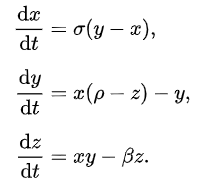
After setting up some loops, extra parameters, and getting all the right matrix dimensions to match, I obtained a nice plot showing solutions to the Lorenz equations for varying values of ρ and initial conditions:
Figure 2: Solutions for the Lorenz system with varying ρ and initial conditions. Initial conditions are plotted as black points, and their respective trajectories are differentiated as red and blue lines.
Two initial conditions were used in all solutions shown; <1, 1, 1>, and <2, 2, 2>.
For the uninitiated - the lower-left plot in Figure 2 shows one of the most interesting properties of "chaotic" systems. While the initial conditions and paths start very close to each other, the paths quickly diverge from one another and lead to very different solutions over time. This behavior is the "chaos" referred to in "chaos theory" and "chaotic systems". Small differences in the initial conditions of a system can lead to dramatically different behavior over time.
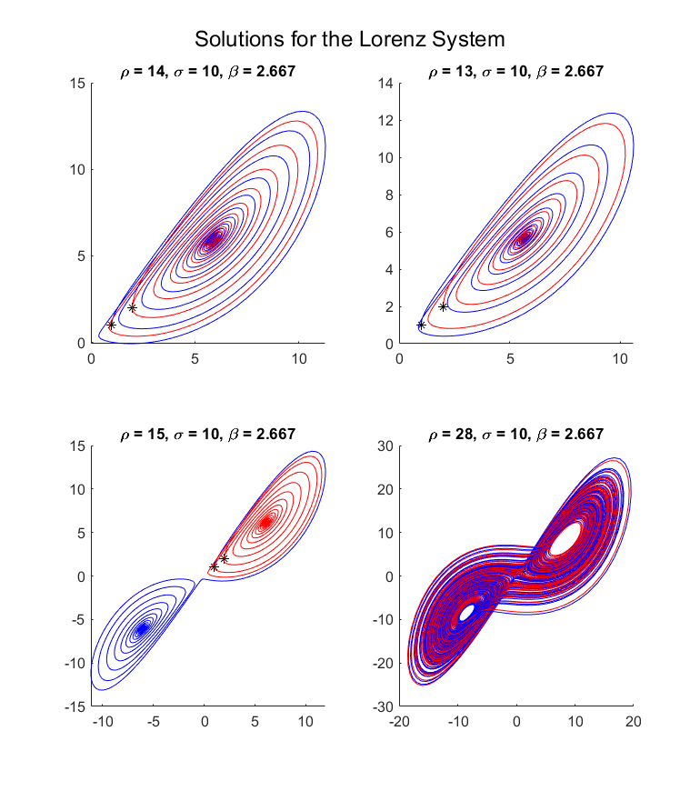
I'm not sure if the "butterfly" in the term "butterfly effect" came from the Lorenz system, but viewing these solutions in the X-Z plane (state variable 1 and 3) yields the prototypical butterfly shape that this system is known for:
Figure 3: Lorenz solutions viewed in the X-Z plane
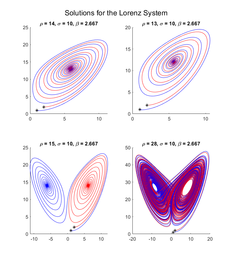
Here's a nice "isometric"-ish viewpoint to highlight that these are 3 dimensional paths:
Figure 4: The Lorenz system from an "isometric"-ish viewpoint
Now that I have the general Lorenz system generating well in MATLAB, it is time for something more interesting. If you haven't seen Professor Steve Brunton's YouTube channel yet, I would definitely recommend checking it out.
Professor Brunton and his lab performs research in a field of controls engineering that I am very interested in; data-driven control. This field applies machine-learning and data science techniques to analyze dynamical systems and develop control algorithms. Since computational power and data are now readily available, non-linear dynamical systems which previously appeared intractable to control, now appear possible.
Anyways, from the paper Chaos as an Intermittently Forced Linear System[1], data-driven techniques are used to linearize the Lorenz system in a higher-dimensional coordinate system. I chose to write my own MATLAB implementation in order to attempt to understand some of the data-driven techniques used and their applicability to controls engineering.
The paper implements a new algorithm, named HAVOK by the paper, for approximating the Koopman operator. From my limited view into the field of data-driven control, attempting to approximate the Koopman operator is a very active field in S.O.T.A controls engineering. The Koopman operator, developed by Bernard Koopman[2], showed that non-linear dynamics could be linearized (caveat: you need an infinite-length vector of all measurements).
The HAVOK algorithm begins by building a Hankel Matrix of time-delayed measurements of 1-variable (x in this case) of the Lorenz system. The "time-delayed" aspect is important here - I'll cover that later. The MATLAB code to build this Hankel matrix, and it's mathematical representation are shown in Figure 5 below.
    %% HAVOK BEGIN

    max_stack_size = 1000;
    r = 15;
    H = zeros(max_stack_size, size(c1, 1) - max_stack_size);

    %% BUILD HANKEL MATRIX
    for k = 1:max_stack_size

        H(k, :) = c1(k:end-max_stack_size-1+k, 1);

    end
Figure 5: First step of HAVOK. A Hankel matrix of time-delay measurements of a single variable is constructed. Note the trimming of the measurement vector; the variable has a total of m measurements, yet the Hankel has only p-columns and q-rows so that even time-delay measurement lengths can be established. The variable "max_stack_size" is used to control both p and q. This code was produced from the book Data-Driven Science and Engineering[3]
After constructing the Hankel matrix, the next step in the HAVOK algorithm is to compute the singular-value decomposition of the Hankel Matrix. Computing the singular-value decomposition on the time-delay measurements located in the Hankel matrix will allow us to separate the dominant time and spatial modes of the measurement (in the context of this SVD, since both the rows and columns are time-series of x, I'm assuming both U and V will be correlated with the time-modes of x. Since there are more columns located within the Hankel matrix, the V matrix will be more interesting and I would expect capture more variation). MATLAB allows for a quick SVD calculation:
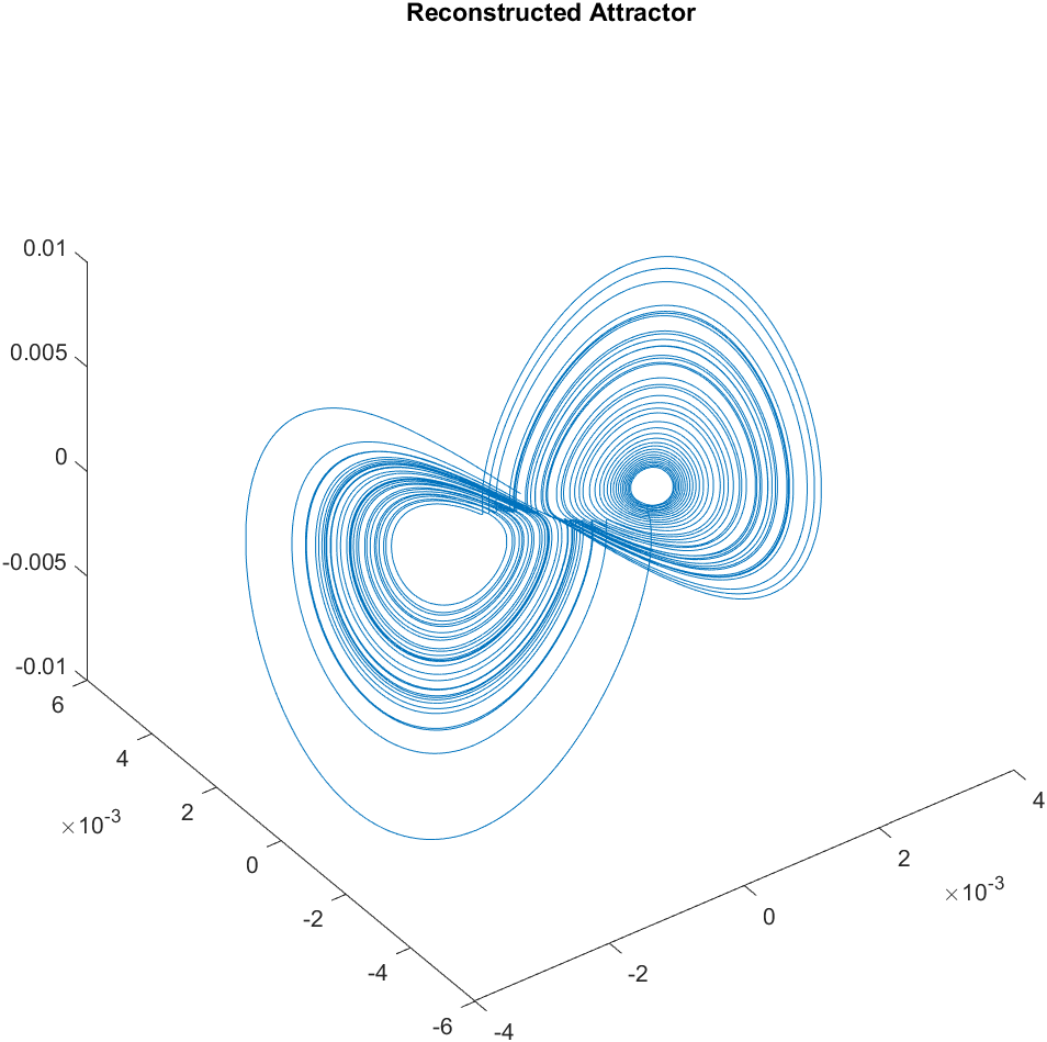
With the SVD now calculated, it is possible to reconstruct the original attractor from these time-delay coordinates. From Taken's Embedding Theorem, and since we chose a good-measurement (the x-coordinate) in this case, within the time-delay measurements of x there is enough information to be able to reconstruct a new attractor which is diffeomorphic (don't understand this too well: I assume this means bijective?) to the original Lorenz system. The MATLAB code and reconstructed attractor are shown in Figure 6 below.
    %% PLOT THE RECONSTRUCTED ATTRACTOR
    %time-delay coordinates are enough to embed the attractor by
    %Takens-embedding theorem

    figure(2)
    v_time_delay_1 = V(:, 1)';
    v_time_delay_2 = V(:, 2)';
    v_time_delay_3 = V(:, 3)';
    plot3(v_time_delay_1, v_time_delay_2, v_time_delay_3);
    title('Reconstructed Attractor');
Figure 6: The reconstructed attractor from the time-delay coordinates created by the SVD of the Hankel Matrix
As I understand this, this is an amazing property of this chaotic system. With only a time-series of a single measurement we can re-create and plot the chaotic behavior of the original system. In controls engineering, there are many variables which are unobservable (i.e. fluid flow velocities, pressures, etc.), yet this shows that with the measurements of a single variable (i.e. pressure at the surface of a wing), some information can be gleamed of these unobservable variables. If there were some known functions which could map this reconstructed attractor to the original Lorenz system (hinting at Koopman theory here?), the measurements of a single variable would allow for prediction of the unobservables of the original system.
The full MATLAB code used to generate these solutions and plots is available here.